Finals Week 1

Here's the detail for Week 1 of the Finals and the road thereafter.

(The base image comes from www.wikipedia.com.)

And the Last Shall be First (At Least Occasionally)

So far we've learned that handicap-adjusted margins appear to be normally distributed with a mean of zero and a standard deviation of 37.7 points. That means that the unadjusted margin - from the favourite's viewpoint - will be normally distributed with a mean equal to minus the handicap and a standard deviation of 37.7 points. So, if we want to simulate the result of a single game we can generate a random Normal deviate (surely a statistical contradiction in terms) with this mean and standard deviation.

Alternatively, we can, if we want, work from the head-to-head prices if we're willing to assume that the overround attached to each team's price is the same. If we assume that, then the home team's probability of victory is the head-to-head price of the underdog divided by the sum of the favourite's head-to-head price and the underdog's head-to-head price.

So, for example, if the market was Carlton $3.00 / Geelong $1.36, then Carlton's probability of victory is 1.36 / (3.00 + 1.36) or about 31%. More generally let's call the probability we're considering P%.

Working backwards then we can ask: what value of x for a Normal distribution with mean 0 and standard deviation 37.7 puts P% of the distribution on the left? This value will be the appropriate handicap for this game.

Again an example might help, so let's return to the Carlton v Geelong game from earlier and ask what value of x for a Normal distribution with mean 0 and standard deviation 37.7 puts 31% of the distribution on the left? The answer is -18.5. This is the negative of the handicap that Carlton should receive, so Carlton should receive 18.5 points start. Put another way, the head-to-head prices imply that Geelong is expected to win by about 18.5 points.

With this result alone we can draw some fairly startling conclusions.

In a game with prices as per the Carlton v Geelong example above, we know that 69% of the time this match should result in a Geelong victory. But, given our empirically-based assumption about the inherent variability of a football contest, we also know that Carlton, as well as winning 31% of the time, will win by 6 goals or more about 1 time in 14, and will win by 10 goals or more a litle less than 1 time in 50. All of which is ordained to be exactly what we should expect when the underlying stochastic framework is that Geelong's victory margin should follow a Normal distribution with a mean of 18.8 points and a standard deviation of 37.7 points.

So, given only the head-to-head prices for each team, we could readily simulate the outcome of the same game as many times as we like and marvel at the frequency with which apparently extreme results occur. All this is largely because 37.7 points is a sizeable standard deviation.

Well if simulating one game is fun, imagine the joy there is to be had in simulating a whole season. And, following this logic, if simulating a season brings such bounteous enjoyment, simulating say 10,000 seasons must surely produce something close to ecstasy.

I'll let you be the judge of that.

Anyway, using the Wednesday noon (or nearest available) head-to-head TAB Sportsbet prices for each of Rounds 1 to 20, I've calculated the relevant team probabilities for each game using the method described above and then, in turn, used these probabilities to simulate the outcome of each game after first converting these probabilities into expected margins of victory.

(I could, of course, have just used the line betting handicaps but these are posted for some games on days other than Wednesday and I thought it'd be neater to use data that was all from the one day of the week. I'd also need to make an adjustment for those games where the start was 6.5 points as these are handled differently by TAB Sportsbet. In practice it probably wouldn't have made much difference.)

Next, armed with a simulation of the outcome of every game for the season, I've formed the competition ladder that these simulated results would have produced. Since my simulations are of the margins of victory and not of the actual game scores, I've needed to use points differential - that is, total points scored in all games less total points conceded - to separate teams with the same number of wins. As I've shown previously, this is almost always a distinction without a difference.

Lastly, I've repeated all this 10,000 times to generate a distribution of the ladder positions that might have eventuated for each team across an imaginary 10,000 seasons, each played under the same set of game probabilities, a summary of which I've depicted below. As you're reviewing these results keep in mind that every ladder has been produced using the same implicit probabilities derived from actual TAB Sportsbet prices for each game and so, in a sense, every ladder is completely consistent with what TAB Sportsbet 'expected'.

The variability you're seeing in teams' final ladder positions is not due to my assuming, say, that Melbourne were a strong team in one season's simulation, an average team in another simulation, and a very weak team in another. Instead, it's because even weak teams occasionally get repeatedly lucky and finish much higher up the ladder than they might reasonably expect to. You know, the glorious uncertainty of sport and all that.

Consider the row for Geelong. It tells us that, based on the average ladder position across the 10,000 simulations, Geelong ranks 1st, based on its average ladder position of 1.5. The barchart in the 3rd column shows the aggregated results for all 10,000 simulations, the leftmost bar showing how often Geelong finished 1st, the next bar how often they finished 2nd, and so on.

The column headed 1st tells us in what proportion of the simulations the relevant team finished 1st, which, for Geelong, was 68%. In the next three columns we find how often the team finished in the Top 4, the Top 8, or Last. Finally we have the team's current ladder position and then, in the column headed Diff, a comparison of the each teams' current ladder position with its ranking based on the average ladder position from the 10,000 simulations. This column provides a crude measure of how well or how poorly teams have fared relative to TAB Sportsbet's expectations, as reflected in their head-to-head prices.

Here are a few things that I find interesting about these results:

• St Kilda miss the Top 4 about 1 season in 7.
• Nine teams - Collingwood, the Dogs, Carlton, Adelaide, Brisbane, Essendon, Port Adelaide, Sydney and Hawthorn - all finish at least once in every position on the ladder. The Bulldogs, for example, top the ladder about 1 season in 25, miss the Top 8 about 1 season in 11, and finish 16th a little less often than 1 season in 1,650. Sydney, meanwhile, top the ladder about 1 season in 2,000, finish in the Top 4 about 1 season in 25, and finish last about 1 season in 46.
• The ten most-highly ranked teams from the simulations all finished in 1st place at least once. Five of them did so about 1 season in 50 or more often than this.
• Every team from ladder position 3 to 16 could, instead, have been in the Spoon position at this point in the season. Six of those teams had better than about a 1 in 20 chance of being there.
• Every team - even Melbourne - made the Top 8 in at least 1 simulated season in 200. Indeed, every team except Melbourne made it into the Top 8 about 1 season in 12 or more often.
• Hawthorn have either been significantly overestimated by the TAB Sportsbet bookie or deucedly unlucky, depending on your viewpoint. They are 5 spots lower on the ladder than the simulations suggest that should expect to be.
• In contrast, Adelaide, Essendon and West Coast are each 3 spots higher on the ladder than the simulations suggest they should be.

(In another blog I've used the same simulation methodology to simulate the last two rounds of the season and project where each team is likely to finish.)

Game Cadence

If you were to consider each quarter of football as a separate contest, what pattern of wins and losses do you think has been most common? Would it be where one team wins all 4 quarters and the other therefore losses all 4? Instead, might it be where teams alternated, winning one and losing the next, or vice versa? Or would it be something else entirely?

The answer, it turns out, depends on the period of history over which you ask the question. Here's the data:

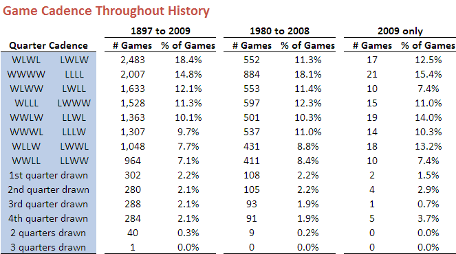
So, if you consider the entire expanse of VFL/AFL history, the egalitarian "WLWL / LWLW" cadence has been most common, occurring in over 18% of all games. The next most common cadence, coming in at just under 15% is "WWWW / LLLL" - the Clean Sweep, if you will. The next four most common cadences all have one team winning 3 quarters and the other winning the remaining quarter, each of which such cadences have occurred about 10-12% of the time. The other patterns have occurred with frequencies as shown under the 1897 to 2009 columns, and taper off to the rarest of all combinations in which 3 quarters were drawn and the other - the third quarter as it happens - was won by one team and so lost by the other. This game took place in Round 13 of 1901 and involved Fitzroy and Collingwood.

If, instead, you were only to consider more recent seasons excluding the current one, say from 1980 to 2008, you'd find that the most common cadence has been the Clean Sweep on about 18%, with the "WLLL / "LWWW" cadence in second on a little over 12%. Four other cadences then follow in the 10-11.5% range, three of them involving one team winning 3 of the 4 quarters and the other the "WLWL / LWLW" cadence.

In short it seems that teams have tended to dominate contests more in the 1980 to 2008 period than had been the case historically.

(It's interesting to note that, amongst those games where the quarters are split 2 each, "WLWL / LWLW" is more common than either of the two other possible cadences, especially across the entire history of footy.)

Turning next to the current season, we find that the Clean Sweep has been the most common cadence, but is only a little ahead of 5 other cadences, 3 of these involving a 3-1 split of quarters and 2 of them involving a 2-2 split.

So, 2009 looks more like the period 1980 to 2008 than it does the period 1897 to 2009.

What about the evidence for within-game momentum in the quarter-to-quarter cadence? In other words, are teams who've won the previous quarter more or less likely to win the next?

Once again, the answer depends on your timeframe.

Across the period 1897 to 2009 (and ignoring games where one of the two relevant quarters was drawn):

• teams that have won the 1st quarter have also won the 2nd quarter about 46% of the time
• teams that have won the 2nd quarter have also won the 3rd quarter about 48% of the time
• teams that have won the 3rd quarter have also won the 4th quarter just under 50% of the time.

So, across the entire history of football, there's been, if anything, an anti-momentum effect, since teams that win one quarter have been a little less likely to win the next.

Inspecting the record for more recent times, however, consistent with our earlier conclusion about the greater tendency for teams to dominate matches, we find that, for the periods 1980 to 2008 (and, in brackets, for 2009):

• teams that have won the 1st quarter have also won the 2nd quarter about 52% of the time a little less in 2009)
• teams that have won the 2nd quarter have also won the 3rd quarter about 55% of the time (a little more in 2009)
• teams that have won the 3rd quarter have also won the 4th quarter just under 55% of the time (but only 46% for 2009).

In more recent history then, there is evidence of within-game momentum.

All of which would lead you to believe that winning the 1st quarter should be particularly important, since it gets the momentum moving in the right direction right from the start. And, indeed, this season that has been the case, as teams that have won matches have also won the 1st quarter in 71% of those games, the greatest proportion of any quarter.

July - When a Fan's Thoughts Turn to Tanking

Most major Australian sports have their iconic annual event. Cricket has its Boxing Day test, tennis and golf have their respective Australian Opens, rugby league has the State of Origin series, rugby union the Bledisloe, and AFL, it now seems, has the Tanking Debate, usually commencing near Round 15 or 16 and running to the end of the season proper.

The T-word has been all over the Melbourne newspapers and various footy websites this week, perhaps most startlingly in the form of Terry Wallace's admission that in Round 22 of 2007 in the Tigers clash against St Kilda, a game in which the Tigers led by 3 points at the final change but went on to lose by 10 points:

"while he had not "tanked" during the Trent Cotchin game in Round 22, 2007, he had let the contest run its natural course without intervention"

That stain on the competition's reputation (coupled, I'll admit, with he realisation that the loss cost MAFL Investors an additional return of about 13% for that year) makes it all the more apparent to me that the draft system, especially the priority draft component, must change.

Here's what I wrote on the topic - presciently as it turns out - in the newsletter for Round 19 of 2007.

Tanking and the Draft

If you’re a diehard AFL fan and completely conversant with the nuances of the Draft, please feel free to skip this next section of the newsletter.

I thought that a number of you might be interested to know why, in some quarters, there’s such a fuss around this time of year about “The Draft” and its potential impact on the commitment levels of teams towards the bottom of the ladder.

The Draft is, as Wikipedia puts it, the “annual draft of young talent” into the AFL that takes place prior to the start of each season. In the words of the AFL’s own website:

"In simple terms, the NAB AFL Draft is designed to give clubs which finished lower on the ladder the first opportunity to pick the best new talent in Australia. At season's end, all clubs are allocated draft selections. The club that finished last receives the first selection, the second last team gets the second selection and so on until the premier receives the 16th selection."

So, here’s the first issue: towards season’s end, those teams for whom all hopes of a Finals berth have long since left the stadium find that there’s more to be gained by losing games than there is by winning them.

Why? Well say, for example, that Richmond suddenly remembered what the big sticks are there for and jagged two wins in the last four games, leaping a startled Melbourne in the process, relegating them to position Spoon. The Tigers’ reward for such a stunning effort would be to (possibly – see below) hand Melbourne the sweetest of draft plums, the Number 1 draft pick, while relegating themselves to the Number 2 pick. Now, in truth, over the years, Number 1 picks have not always worked out better than Number 2 picks, but think about it this way: isn’t it always nicer to have first hand into the Quality Assortment?

Now entereth the notion of Priority Picks, which accrue to those teams who have demonstrated season-long ineptitude to the extent that they’ve accumulated fewer than 17 points over its duration. They get a second draft pick prior to everyone else’s second draft pick and then a third pick not that long after, once all the other Priority Picks have taken place. So, for example, if a team comes last and wins, say, four games, it gets Pick #1, Pick #17 (their Priority pick, immediately after all the remaining teams have had their first pick) and then Pick #18 (their true second round Pick). If more than one team is in entitled to Priority Picks then the Picks are taken in reverse ladder order.

Still with me?

Now, the final twist. If a team has proven its footballing inadequacy knows not the bounds of a single year, having done so by securing fewer than 17 points in each of two successive seasons, then it gets its Priority Pick before anyone else gets even their first round pick. Once again, if more than one team is in this situation, then the tips are taken in reverse ladder order.

So, what’s the relevance to this year? Well, last year Carlton managed only 14 points and this year they’re perched precipitously on 16 points. If they lose their next four games, their first three draft picks will be #1 (their Priority Pick), #4 (their first round pick), and #20 (their second round pick); if they win or even draw one or more of their remaining games and do this without leaping a ladder spot, their first three draft picks will be #3, #19 and #35. Which would you prefer?

I find it hard to believe that a professional footballer or coach could ever succumb to the temptation to “tank” games (as it’s called), but the game’s administrators should never have set up the draft process in such a way that it incites such speculation every year around this time.

I can think of a couple of ways of preserving the intent of the current draft process without so blatantly rewarding failure and inviting suspicion and rumour. We’ll talk about this some more next week.

*****

In the following week's newsletter, I wrote this:

Revising the Draft

With the Tigers and the Dees winning last week, I guess many would feel that the “tanking” issue has been cast aside for yet another season. Up to a point, that’s probably a fair assessment, although only a win by the Blues could truly muffle all the critics.

Regardless, as I said last week, it’s unfair to leave any of the teams in a position where they could even be suspected of putting in anything other than a 100% effort.

I have two suggestions for changes to the draft that would broadly preserve its intent but that would also go a long way to removing much of the contention that currently exists.

(1) Randomise the draft to some extent. Sure, give teams further down the ladder a strong chance of getting early draft picks, but don’t make ladder position completely determine the pick order. One way to achieve this would be to place balls in an urn with the number of balls increasing as ladder position increased. So, for example, the team that finished 9th might get 5 balls in the urn; 10th might get 6 balls, and so on. Then, draw from this urn to determine the order of draft picks.

Actually, although it’s not strictly in keeping with the current spirit of the draft, I’d like to see this system used in such a way that marginally more balls are placed in the urn for teams higher up the ladder to ensure that all teams are still striving for victory all the way to Round 22.

(2) Base draft picks on ladder position at the end of Round 11, not Round 22.

Sides that are poor performers generally don’t need 22 rounds to prove it; 11 rounds should be more than enough. What’s more, I reckon that it’s far less likely that a team would even consider tanking say rounds 9, 10 and 11 when there’s still so much of the season to go that a spot in the Finals is not totally out of the question. With this approach I’d be happy to stick with the current notion that 1st draft pick accrues to the team at the foot at the ladder.

Under either of these new draft regimes, the notion of Priority Picks has to go. Let’s compensate for underperformance but not lavish it with silken opportunity.

****

My opinion hasn't changed. The changes to the draft for the next few years that have been made to smooth the entry of the Gold Coast into the competition probably mean that we're stuck with a version of the draft we have now for the next few years. After that though, we do have to fix it because it is broken.

The Differential Difference

Though there are numerous differences between the various football codes in Australia, two that have always struck me as arbitrary are AFL's awarding of 4 points for a victory and 2 from a draw (why not, say, pi and pi/2 if you just want to be different?) and AFL's use of percentage rather than points differential to separate teams that are level on competition points.

I'd long suspected that this latter choice would only rarely be significant - that is, that a team with a superior percentage would not also enjoy a superior points differential - and thought it time to let the data speak for itself.

Sure enough, a review of the final competition ladders for all 112 seasons, 1897 to 2008, shows that the AFL's choice of tiebreaker has mattered only 8 times and that on only 3 of those occasions (shown in grey below) has it had any bearing on the conduct of the finals.

Historically, Richmond has been the greatest beneficiary of the AFL's choice of tiebreaker, being awarded the higher ladder position on the basis of percentage on 3 occasions when the use of points differential would have meant otherwise. Essendon and St Kilda have suffered most from the use of percentage, being consigned to a lower ladder position on 2 occasions each.

There you go: trivia that even a trivia buff would dismiss as trivial.