Simulating SuperMargin Wagering

Season 2013 has been a good one, so far, for SuperMargin wagering, which led me to ponder why that might be the case. More generally, I wondered if we could define the characteristics of a season and of the predictive algorithm that we're using for selecting wagers, which are most propitious for this form of wagering.

ASSUMPTIONS

We first need to make some assumptions about the underlying process that is generating game outcomes.

For today's blog I'm going to assume that the final game margin is distributed normally with mean equal to the negative of the Bookmaker's handicap and with some constant variance. Across different simulation runs I'll vary the value of this variance to determine the extent to which it affects the accuracy with which the correct SuperMargin bucket can be expected to be chosen, and the extent to which it affects the expected returns to wagering.

My second assumption relates to the behaviour of my predictive algorithm. Its margin predictions, I'll assume, are also normally distributed with a mean equal to the negative of the Bookmaker's handicap for the game and with a constant variance, set independently of the variance in game outcomes. I'll also vary the value of the variance that I use to model the predictive algorithm's outcomes across different scenario replications.

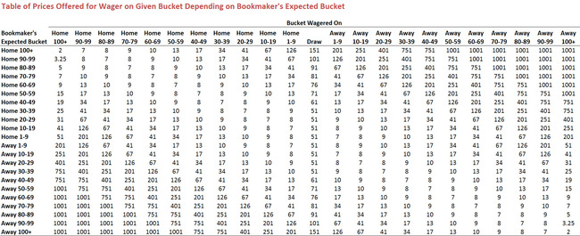
Lastly, because I want to estimate not just the expected accuracy of the predictive algorithm but also its expected return from wagering in the SuperMargin market, I need a lookup table to provide an assumed price for a successful wager on a particular bucket given the Bookmaker's assessment of the likely game margin. For this purpose I used recent TAB Sportsbet markets for SuperMargin wagering and, after some interpolation (and even some scandalous extrapolation), came up with this:

OUTLINE OF THE SIMULATION PROCESS

In outline, here are the steps I took to simulate the results for a single run of the simulation:

1. Select a variance to use for game outcomes for the current scenario (actually I selected a standard deviation, sigma, but this amounts to the same thing). For the scenarios I ran to estimate the accuracy of the predictive models I allowed sigma to vary from 30 to 40. So, for example, for the entirety of the first simulation run, I set sigma to 30.
2. Select a variance to use for the predictive algorithm (again, in reality, I chose a standard deviation, sigma). For this same set of scenarios I allowed the sigma for the predictive algorithm to vary from 0 (in which case the predictive algorithm always selects the negative of the Bookmaker handicap) to 100 (in which case the predictive algorithm might as well be throwing darts - albeit unbiased ones).
3. Generate an expected game margin (for this purpose I selected one handicap, at random, from those of the TAB Sportsbet Bookmaker across all games from 2006 to the present).
4. Generate a prediction from the predictive algorithm (using the assumption of normality described earlier)
5. Generate an outcome for the game (also using the assumption of normality described earlier)
6. Convert the expected, predicted and actual game margins to SuperMargin buckets
7. Determine whether or not the predicted bucket matches the actual bucket
8. Repeat the process above 100,000 times for each set of outcome and predictive algorithm variances 

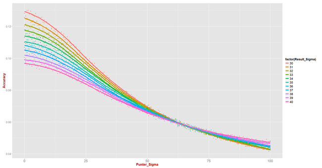
The result of these simulations is summarised in this chart:

Each line summarises the results for a given value of the outcome variance as we alter the sigma for the predictive algorithm (or, as I've labelled it here, the "Punter"). The key findings are that: 

• For values of sigma for the predictive algorithm less than about 60 points per game, the less variable the outcome of games, the more accurate we can expect a predictive algorithm like the one I've posited  - which, for example, is unbiased - to be. Curiously, the opposite is true for values of sigma for the predictive algorithm above about 60. I speculate that this is because larger values of sigma mean the predictive algorithm makes more predictions in the extreme, 100+ buckets, which allows it to predict these upsets more often than more timid predictive algorithms. To be clear though, the difference is quite small - no more than about one-half a percentage point
• For a given level of variability in game outcomes, the less variable the predictions made by our predictive algorithm the more accurate we can expect it to be
• In percentage point terms, the increases in predictive accuracy for reduced variability in outcomes are most pronounced when the variability of our own predictions is smallest. For example when we set the sigma for our predictions to zero (the leftmost part of the curves), the difference in the expected accuracy of our predictions when the sigma for outcomes is 40 points per game as compared to when it's 30 points per game is over 3 percentage points - from just under 10% to about 13%. 

EXPECTED WAGERING PERFORMANCE

It's one thing to be accurate, but usually another thing entirely to be profitable in wagering. We can imagine, for example, one algorithm that wagers only on teams in the head-to-head market priced at under $2 and which collects 40% of the time, and compare it to another algorithm that wagers only on teams in the head-to-head market priced at over $4 and which collects "only" 30% of the time. In a narrow sense that first algorithm is more accurate, but I know which algorithm I'd rather be using to wager.

So, by considering only the accuracy of the variously simulated predictive algorithms in variously unpredictable outcome environments, we've done only half the job.

To complete the task we need to assess wagering profitability. It turns out that profit is extraordinarily variable, so much so that I needed to perform 1 million replications for each combination of outcome and predictive algorithm variability in order to produce estimates with an acceptable level of precision. That, of course, meant each scenario took longer to run, so I restricted the range of variances that I considered. For outcome variability I explored sigmas only in the range 30 to 35, and for predictive variability I explored only sigmas in the range 0 to 20. (I discuss the empirical rationale for these ranges later.)

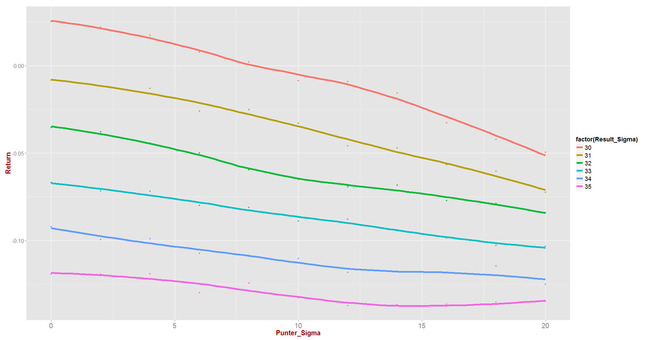
The results of these simulations are summarised in the following chart:

We can see from this chart that:

• Lower outcome variability leads to higher profitability for any given level of predictive variability
• The returns to reduced predictive variability increase as outcome variability falls (ie the slope of the lines gets steeper with smaller outcome variability)
• Profitability is only expected for outcome variability of 30 points per game and for predictive variability of less than about 8 points per game

PRACTICAL IMPLICATIONS FOR WAGERING

As a first step in assessing the practical implications of these results we need to determine, empirically, what values of outcome variability are plausible. If we assume that the TAB Bookmaker's handicaps in each game are an unbiased estimate of the true expected game margin, then we can estimate outcome variability by calculating the standard deviation of handicap-adjusted game results. In other words, for each game we add the Bookmaker's handicap to the actual game margin to calculate a handicap-adjusted margin (HAMs), and then calculate the standard deviation of these HAMs.

Over the period from 2006 to the present that yields a standard deviation of about 37 points per game, which is distressingly distant from the 30 we were hoping for. If, however, we restrict our analysis to the current season only (ie 2013), the standard deviation drops to 33.1 points per game, which is lower than the result for any single season across the entire span we've been considering. This, I suspect, is part of the reason we've been doing so well on SuperMargin wagering this season.

Under the assumption that the Bookmaker we're facing in the market is an unbiased judge of the true expected game margin, it's no surprise that our simulations suggest the best strategy to follow is to wager on the bucket in which his expected game margin falls. This bucket will have the lowest price and, consistent with the analyses we've undertaken previously on the head-to-head market, is therefore likely to carry the least overround. That makes it the most profitable bucket and, in extreme circumstances, when outcome variability is very small, makes it a net profitable proposition. (I do wonder, however, if a Bookmaker, faced with a prolonged period of reduced outcome variability would simply stop offering a $7 price for the expected bucket. Perhaps we'll see.)

Of course if the Bookmaker is not unbiased - and, again, we've had reason to speculate that this might be the case before - then some benefit might be gained by a punter with a little bias or variability of his or her own. I'll investigate this possibility in a future blog.

For now though, suffice it for me to present the figures for the predictive variability of some of the MAFL Margin Predictors. I've calculated these, only for the 2013 season, and as the standard deviation of their handicap-adjusted predictions.

Bookie_LPSO has the smallest sigma at just 5.7 points per game, with Bookie_3 (6.8), RSMP_Weighted (7.1) and RSMP_Simple (8.1) the next smallest. Win_3 has the largest sigma at 18.1 points per game, though Win_7 (17.6) and the four H2H Predictors (16.7 to 17.0) also have large sigmas. Combo_NN2 has a sigma of 15.3 points per game.