Yet Another Look at Bookmaker Overround

Lately I've been pondering the challenge of determining how much overround the TAB Bookmaker has embedded in the head-to-head prices of each team in an AFL contest. 

(Those of you with an absence of fondness for algebra might want to skip ahead a few section while I amble through the maths behind today's blog.)

Overround is more usually defined in relation to the head-to-head prices for both teams, where it's customarily defined as (ignoring draws):

Total Overround, T = 1/m1 + 1/m2 - 1 (where m1 and m2 are the head-to-head prices for the two teams)

The total overround in a market is a measure of how competitive that market is. In a typical game in recent times the TAB Bookmaker has set head-to-head prices such that T is about 5-6%, which is down by about 1 to 1.5% points over the past couple of years reflecting increased competition from other bookmakers in Australia and from services such as Betfair.

At the level of a team I've defined overround (Ov) via the following relation:

m = 1/p(1+Ov) (where p is the victory probability, as assessed by the Bookmaker, of the team in question)

This makes overround the link between the Bookmaker's probability assessment, p, and his market price, m. More specifically, since the fair price for a team with a victory probability of p is 1/p (because at that price a wager on the team would be a breakeven proposition) the factor 1/(1+Ov) deflates the market price and serves as a buffer for the Bookmaker, protecting him against his own underestimation of a team's true chances.

We can move between the overround on each team and the total overround in the market as a whole via the following relation:

T = (Ov1 - Ov2) / m1(1+Ov1) + Ov2

That's all very well, but we observe only the Bookmaker's market prices, m1 and m2, and so need to infer or describe p or Ov for one of the teams. (Once we know p for one team, the victory probability for the other team must be 1-p since I'm ignoring draws, and once we know Ov for one team, the overround for the other team can be derived based on the equation for T shown above.)

We can proceed then either by describing how Ov is determined by the Bookmaker for one team and then inferring p for both teams, or by describing a relationship between T and m and p for one team, and then inferring Ov for each team. 

OVERROUND ALLOCATION TO EACH TEAM

In previous blogs I've pursued the first of these options and posited what I've claimed to be plausible theoretical equations for Ov, then derived p and measured its empirical support by way of probability scores when it's applied to actual games between 2007 and 2012. 

For most of the past seven years, though there's no particular reason to believe that it's the way Bookmakers actually behave in practice, I've followed the precedent set by much of the extant literature and assumed that overround is levied equally on both teams. If this is the case then:

Ov1 = Ov2 = T

and we can infer the Bookmaker's probability assessment of the victory chances of, say, team 1, by using:

Victory Probability for Team 1, p1 = m2 / (m1 + m2)

(We can calculate the implicit victory probability assessment for Team 2 analogously.)

The overround baked into Team 1's (and Team 2's) price is then just T, and we have

mi = 1/pi (1+T)

That's one approach to defining Ov, but in recent posts I've demonstrated that levying overround on both teams equally leads to asymmetric outcomes in terms of the calibration error against which a Bookmaker is protected. Specifically, he runs the risk of offering a market price on the underdog that has negative expectation if his assessment of that team's true victory chances is even a small bit underestimated.

That led me to develop an alternative approach to defining Ov, in which the overround baked into the price of each team was sufficient to provide "cover" for the same sized calibration error on both teams. Given this assumption we derived the following, alternative equations:

Victory Probability for Team 1 = 1/m1 - T/2

Ov1 = (T x m1) /(2 - T x m1)

(Again, the equations for Team 2 can be stated analogously).

I've labelled the two approaches to defining Ov discussed above as Overround-Equalising and Risk-Equalising and, while they've some intuitive appeal, there's no guarantee that either of them is correct. Doubtless, there are other approaches that are also worth pursuing, but that's not my aim today - at least, not directly.

DEFINING A RELATIONSHIP FOR P, M AND T

An alternative to theoretically defining Ov and then deriving p is to posit an equation for p in terms of m and T, assess its empirical validity, and then derive the Ov that it implies. This is the path that I'll pursue in the remainder of this blog, somewhat like the approach I adopted in this earlier blog.

The first task then is to come up with a variety of plausible equations for p as a function of T and m, call them p = g(T,m), and then assess the empirical validity of each function g by calculating the probability score obtained in practice on actual results when we assume that g is the function by which to determine the Bookmaker's true underlying probabilities.

If we assume that the Bookmaker is, among other things, well-calibrated (ie teams that he rates as X% chances will win about X% of the time) then we should prefer those specifications, g, that lead to superior probability scores.

SOME PRACTICAL ISSUES

How well-performed is a predictor for p depends on the metric we use to calculate its performance. For this blog I'll use two metrics:

• Log Probability Score = 1+log2(p) where p is the probability assigned to the winning team, and
• Brier Score = (1-p)2 where p is the probability assigned to the winning team

Also, when we write p = g(T,m) we need to determine to which team the relation applies. For this blog I'll investigate, separately, choosing a function g for the Home team, the Favourite, the Away team, and the Underdog.

A TANGIBLE EXAMPLE

It's easy to get lost in all that algebra (I know I did, and Google Maps was no help at all), so an example of what I'll be doing for this blog might help. Remember, the approach here is to define plausible equations for p and then assess them empirically (and then derive the equation for Ov that they imply).

We know that the Risk-Equalising approach sets p1 = 1/m1 - T/2, so one approach might be to generalise this by defining:

p1 = 1/m1 - T/k

Using actual results - for all games from 2007 to 2012 - we could then determine:

• the value of k that would maximise the Log Probability Score of the resulting predictor
• the value of k - which might be different - that would minimise the Brier score of the resulting predictor

(We can do this because we know the actual result, m1, and T for every game.)

A little more maths allows us to derive that, for this specificatiion of p1: 

• Ov1 = (T x m1) / (k -T x m1)
• Ov2 = (T x m1)(k - 1) / (k (m1 - 1) + T x m1)

So, once we've emprically determined an optimal k we can determine the implicit Bookmaker probabilities for each team, p1 and p2, and the overround embedded in each team's head-to-head price, Ov1 and Ov2.

We can make other assumptions about the form of the equation for p1, parameterising some variable k, and proceed similarly, empirically determining optimal values for k based on optimising some probability score, calculating implicit probabilities for both teams, deriving expressions for Ov1 and Ov2, and then calculating the Overround embedded in each team's head-to-head price in each game.

How about I get on and do that then.

THE RESULTS

I assessed seven different equations for expressing either the Home team's, the Favourite's, the Away team's or the Underdog's implicit probability, p, as a function of its head-to-head price, m, and the total overround in both head-to-head prices in the game, T, using Excel's Solver add-in to determine an optimal k for each.

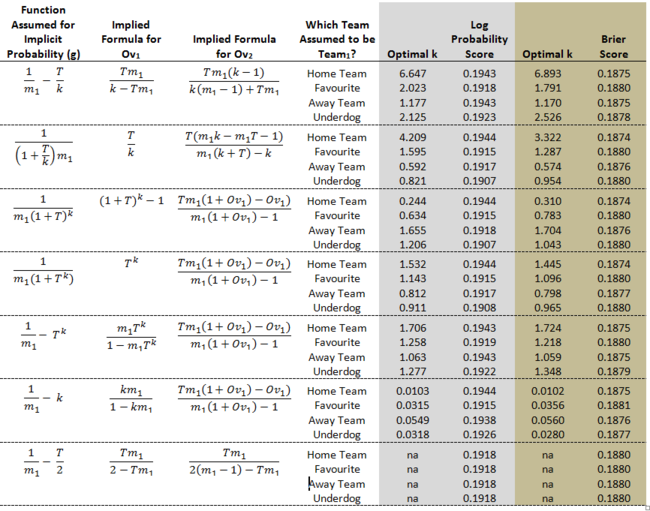
The table below describes those equations for p, the formulae they imply for the overrounds of each team, and the empirically optimal k based on maximising a Log Probability Score or minimising a Brier Score.

Firstly, a few general observations: 

• Setting Team 1 to be the Home team results in superior probability scores, regardless of the formulation selected or whether we prefer the Log Probability Score or the Brier Score.
• Relatively speaking, the Log Probability Score is more discriminating than the Brier Score, regardless of the formulation chosen. Note that this does not necessarily make the Log Probability Score a "better" metric, but it does make it the one I'll prefer in this blog.
• If we define Team 1 to be the Home team and concentrate on the Log Probability Score, there's little to choose amongst the various formulations as they all (aside from the last, which is the Risk-Equalising formulation) produce scores of 0.1943 or 0.1944. Three of the six formulations do not have the Home team overround dependent on its price (ie there's no m1 in the equation for Ov1), which suggests that the assumption of a "flat rate" overround on Home teams is empirically supported.
• In contrast, if we concentrate on the results when the Away team is defined to be Team 1, we find that the formulations with the overround dependent on the Away team price are superior to those where the overround does not depend on m1.
• Taken together, the previous two points suggest that it is reasonable to assume that the overround on the Home team is related only to the total overround in the market (or only loosely related to the Home team's price), whereas the overround on the Away team is very much related to its price as well as to the total overround in the market.

Next, let's go through each of the formulations in turn, and focus on the assumption that Team 1 is the Home team and the Log Probability Score is the preferred metric.

GENERALISATION OF THE RISK-EQUALISING EQUATION

We've derived previously, under the assumption that overround on both teams is set to equalise the risk due to equally-sized calibration errors, that 

p1 = 1/m1 - T/2

In the first formulation for p1 in the table we simply generalise the divisor for T. It turns out that, using this approach, the optimal divisor is about 6.6. The high value for k suggests that Home teams carry much less overround than Away teams.

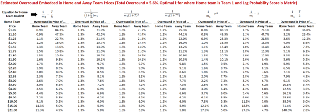
For example, where the Home team is priced at $1.80 and the Away team at $2.00 (and hence T is about 5.6%), the overround embedded in the Home team's price is estimated as being about 1.5% while that in the Away team's price is estimated at 10.4%.

TEAM 1 OVERROUND IS T/k

Recall that we defined p = 1/m(1+Ov), so the second functional form in the table above implies that Ov = T/k, which means that the overround on Team 1 is some fixed proportion, k, of the Total Overround.

Using this approach, the optimal divisor is about 4.2, which again suggests that Home teams carry much less overround than Away teams. For a market where the Total Overround is about 5.6% as we had before, this suggests that overround embedded in the Home team's price is about 1.3% while that in the Away team's price is about 10.7%. 

These embedded overround estimates are very similar to those we calculated for the previous formulation.

TEAM 1 OVERROUND IS (1+T)k - 1

In this specification the optimal value for k turn out to be about one-quarter. With typical values of T in the 4% to 8% range, this makes the overround on the Home team grow very slowly with the growth of Total Overround in the market.

For example, the overround embedded in the Home team price for our theoretical contest with T=5.6% is about 1.3% for the Home team and 10.7% for the Away team, which are once again very similar to previous estimates.

TEAM 1 OVERROUND IS Tk

In this specification the optimal value for k is around 1.5 and the estimated overround embedded in the prices of our theoretical $1.80/$2.00 contest are about 1.2% for the Home team and 10.9% for the Away team, which are again in a similar ballpark.

TEAM 1 OVERROUND IS (m1 x Tk) / (1- m1 x Tk)

Here the optimal k value is 1.706 and the estimated overround for the $1.80/$2.00 contest is 1.3% for the Home team and 10.7% for the Away team. More discerning readers will, by now, be discerning a pattern ...

TEAM 1 OVERROUND IS (k x m1) / (1- k x m1)

In this formulation, the Implicit Probability of the Home team is simply the inverse of the Home team's price less a fixed proportion, regardless of the Total Overround in the market.

The optimal value for that fixed proportion, k, is 0.0103 (or 1.03%) and the estimated overround for the $1.80/$2.00 contest is 1.9% for the Home team and 10.0% for the Away team. This formulation, therefore, assumes the highest embedded overround in the Home team's price, and the lowest embedded overround in the Away team's price of all formulations so far, but it still implies almost 5 times the overround in the Away team's price as in the Home team's.

RISK-EQUALISING APPROACH

Notwithstanding the demonstrably superior predictive powers of implicit probabilities derived using the Risk-Equalising Approach, our results from the current analysis suggest that a number of other formulations are clearly superior to this one. The Log Probability Score for this formulation is just 0.1918, which is considerably smaller than the score of 0.1944 recorded by those other formulations.

ESTIMATED HOME TEAM OVERROUND AT DIFFERENT HOME TEAM PRICES

As I've hinted at during the course of the review of the various formulations just completed - the Risk-Equalising Formulation aside - the similarity of each formulation's Log Probability Scores is reflected in the estimates they provide of the overround embedded in Home and Away team prices as we vary the Home team price for a given Total Overround.

Assuming that the overround embedded in the Home team's price is about one-quarter of the overround embedded in the total market, and that the overround embedded in the Away team's price makes up the difference, seems to be an empirically supported position.

In particular, it seems apparent that larger overrounds tend to be embedded in Away teams' prices as compared to Home teams', whether the Away team is a firm or slight favourite, or a narrow, mild or rank underdog. This, perhaps more than any analysis I've ever done before, provides an empirical rationale for MAFL's obsession with wagering only on Home teams.

If you're betting on Away teams, you're paying a hefty price.