
;)
Modelling AFL Team Scoring
Today's blog is the first in a series that will look at statistically modelling the scoring behaviour of teams in the AFL.
If you're profoundly reductionist about it, you can think about a team's footy score as being the product of the number of scoring shots it creates and the proportion of those scoring shots that it converts into goals.
Put into an equation, which I'll call the Score Equation, that'd be:
Score = Number of Scoring Shots x Conversion Rate x 6 + Number of Scoring Shots x (1 - Conversion Rate)
The first part of the expression on the right-hand side of the equals sign calculates the points scored from goals and the second part calculates the points scored from behinds.
What I want to do with this equation in this blog is attempt to model the expected value of its components to see if I can therefore come up with a predicted score for a given team.
The first thing to note is that, empirically, scoring-shot production and conversion rates are almost uncorrelated. If a team has a day out and racks up a huge number of scoring shots, that team is not substantially more likely to convert a greater (or smaller) proportion of them into goals than the team they flog. Put another way, high-scoring teams tend to be high-scoring because they generate a lot of scoring shots, not because they kick straighter. The actual correlation between scoring shots and conversion rate for all games in the period 1990-2009 is +0.08 and the mean conversion rate is 53.64%.
A chart depicting the empirical relationship between scoring shots and conversion rate over this timeframe appears below and, as well as the lack of correlation between scoring shots and conversion rate, it's interesting to note the constancy of the mean conversion rate and the reduction in the variability of the conversion rate as the number of scoring shots increases.
The reduction in the variability is so great that, for example, we find no games where a team registers 40 scoring shots but converts at a rate less than 30% or at more than 70% - we therefore find no 12.28 or 28.12 score lines in the historical record.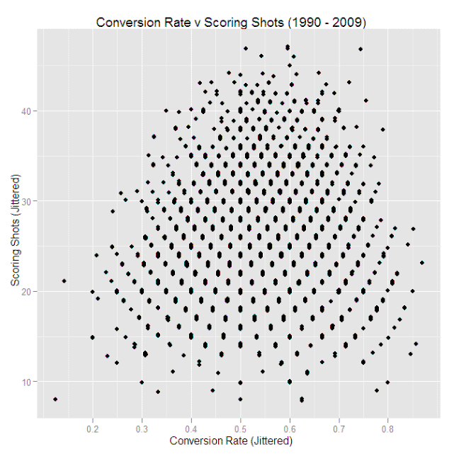
(Because, for a given number of scoring shots, conversion rates can take on only a certain number of fixed values, multiply occurring combinations of scoring shots and conversion rates will be hidden by a standard charting approach. Consequently, I've used a technique known as 'jittering' to produce this chart, which randomly perturbs values a little so that the chart provides a better idea of how many games there are for each combination of scoring shots and conversion rate.)
Knowing that teams convert about 53.64% of their scoring shots we can put that value in place of the Conversion Rate term in the Score Equation.
Next we need to model the other term in that equation: the number of scoring shots. Now the number of scoring shots that a team can expect to generate is a function of how strong it is relative to its opponent - which we can model based on the bookies' view as reflected in the probability of each team's winning implicit in their head-to-head prices - and on each teams' home team status.
The following equation, which has been estimated using the relevant data for the seasons 2006 to 2009, is the result of fitting just such a model:
Expected Number of Scoring Shots = 18.7683 + 13.3395 x Team Probability + 0.7381 x Home Ground Status
(where Team Probability = Opponent Price / (Own Price + Opponent Price) and Home Ground Status = 1 if the team in question is playing at home, and 0 otherwise. The R-squared on this model is about 0.21.)
So, for example, a team that's playing at home and that's an equal favourite can be expected to register 18.7683 + 13.3395 x 0.5 + 0.7381 = 26.2 scoring shots.
Since we know that teams convert about 53.64% of all scoring shots regardless of how many scoring shots they generate we can convert our previous equation for the expected number of scoring shots into an expected score using our Score Equation as follows:
Expected Score = 0.5364 x Expected Number of Scoring Shots x 6 + (1 - 0.5364) x Expected Number of Scoring Shots
This simplifies to what I'll call the Expected Score Equation:
Expected Score = 69.1047 + 49.116 x Team Probability + 2.7176 x Home Ground Status
So, that team playing at home that's an equal favourite can be expected to score 69.1047 + 49.116 x 50% + 2.7176 = 96.4 points. The actual average score of the 48 such teams over the period 2006 to 2009 has been 96.8 points, so clearly we're onto something.
It's interesting that there's a Home Ground Status variable in this model and that its value is statistically significantly different from zero. This means that the bookmaker's price does not completely reflect the value of the home ground advantage - a phenomenon that our MAFL models have exploited for a few years now. In effect, home teams score almost 3 points per game more than they 'should'.
As a final check on the model let's compare its projections with the actual data for seasons 2006 to 2009:
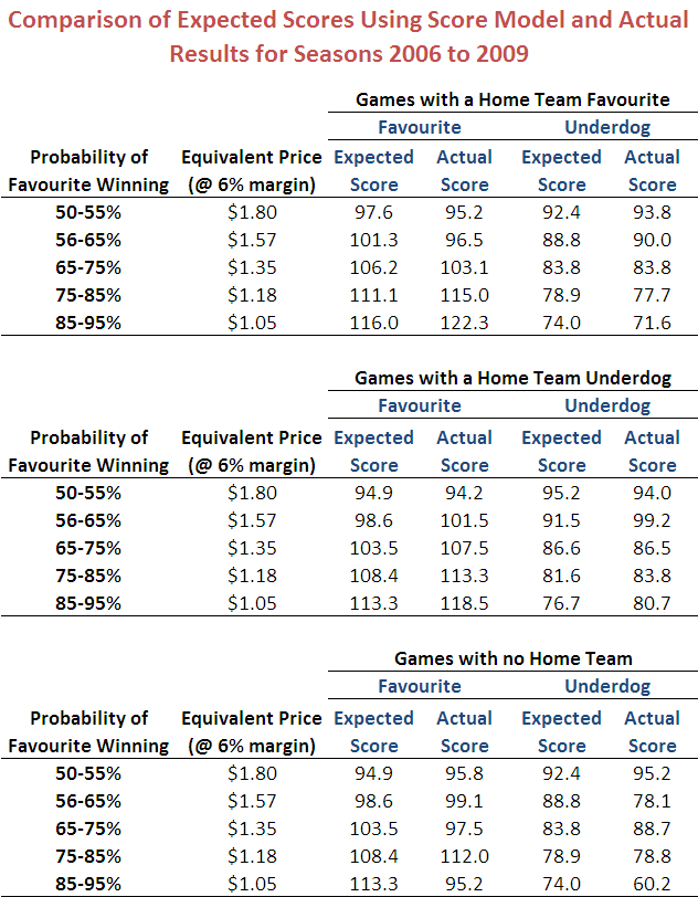
The topmost table refers to matches in which there's a home team favourite and the first row of that table refers to matches where this favourite is priced around $1.80. In such games the Expected Score Equation predicts that favourites will score 97.6 points and underdogs 92.4 points. In actual games of this type, favourites have averaged 95.2 points and underdogs 93.8, so again our predictions are quite close - both within about 2.5% in this case.
For most other rows in this and in the other two tables the differences are generally between 1% and 5% (or about 1 to 5 points), with just a few exceptions. The first exception is for games where there is no home team and where there's a very strong favourite. For these games the differences are around 20%, which can largely be attributed to the fact that there are very few such games - only 5 in fact - so the actual averages are subject to large sample variation. In that same table, the difference between actual and expected scores for underdog teams facing favourites priced around $1.60 is also somewhat large; there are only 25 such games, so sample variation is an issue here too.
One other large difference is a much more interesting one. It's for home team underdogs facing favourites priced around $1.60, where the expected score is almost 8 points lower than the actual average score, which, in this case, is based on 85 games and so is much more reliable. Narrow home team underdogs tend to score more points than bookies expect them too, another anomaly that I think the MAFL Funds have capitalised on over the years.
That's it for this blog. In future blogs we'll make further use of the Score Equation.
 TonyC
TonyC
Reader Comments